Table Calculation Functions
This article introduces table calculation functions and their uses in Tableau. It also demonstrates how to create a table calculation using the calculation editor.
Table calculation functions allow you to perform computations on values in a table.
For example, you can calculate the percent of total an individual sale is for the year, or for several years.
These are the native table calculation functions that can be used in Tableau without an external Analytics Extension.
FIRST( )
Returns the number of rows from the current row to the first row in the partition. For example, the view below shows quarterly sales. When FIRST() is computed within the Date partition, the offset of the first row from the second row is -1.
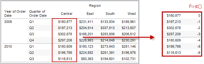
Example
When the current row index is 3, FIRST()
= -2.
INDEX( )
Returns the index of the current row in the partition, without any sorting with regard to value. The first row index starts at 1. For example, the table below shows quarterly sales. When INDEX() is computed within the Date partition, the index of each row is 1, 2, 3, 4..., etc.
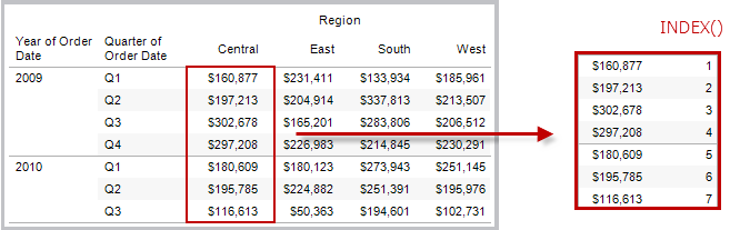
Example
For the third row in the partition, INDEX() = 3.
LAST( )
Returns the number of rows from the current row to the last row in the partition. For example, the table below shows quarterly sales. When LAST() is computed within the Date partition, the offset of the last row from the second row is 5.
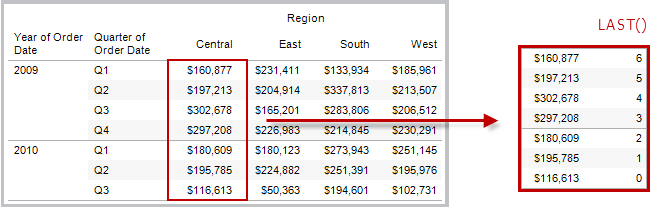
Example
When the current row index is 3 of 7, LAST() = 4.
LOOKUP(expression, [offset])
Returns the value of the expression in a target row, specified as a relative offset from the current row. Use FIRST() + n and LAST() - n as part of your offset definition for a target relative to the first/last rows in the partition. If offset is omitted, the row to compare to can be set on the field menu. This function returns NULL if the target row cannot be determined.
The view below shows quarterly sales. When LOOKUP (SUM(Sales), 2) is computed within the Date partition, each row shows the sales value from 2 quarters into the future.
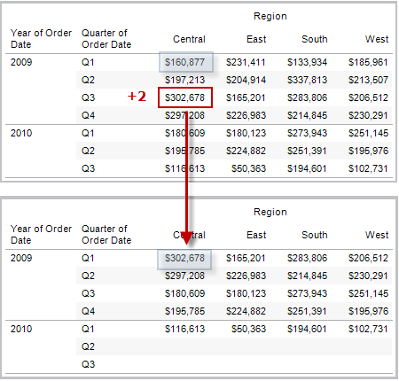
Example
LOOKUP(SUM([Profit]),
FIRST()+2)
computes the SUM(Profit) in the third row of the partition.
MODEL_EXTENSION functions
The model extension functions:
MODEL_EXTENSION_BOOL
MODEL_EXTENSION_INT
MODEL_EXTENSION_REAL
MODEL_EXTENSION_STRING
are used to pass data to a deployed model on an external service such as R, TabPy or Matlab. See Analytics Extensions(Link opens in a new window).
MODEL_PERCENTILE(target_expression, predictor_expression(s))
Returns the probability (between 0 and 1) of the expected value being less than or equal to the observed mark, defined by the target expression and other predictors. This is the Posterior Predictive Distribution Function, also known as the Cumulative Distribution Function (CDF).
This function is the inverse of MODEL_QUANTILE. For information on predictive modelling functions, see How Predictive Modelling Functions Work in Tableau.
Example
The following formula returns the quantile of the mark for sum of sales, adjusted for count of orders.
MODEL_PERCENTILE(SUM([Sales]), COUNT([Orders]))
MODEL_QUANTILE(quantile, target_expression, predictor_expression(s))
Returns a target numeric value within the probable range defined by the target expression and other predictors, at a specified quantile. This is the Posterior Predictive Quantile.
This function is the inverse of MODEL_PERCENTILE. For information on predictive modelling functions, see How Predictive Modelling Functions Work in Tableau.
Example
The following formula returns the median (0.5) predicted sum of sales, adjusted for count of orders.
MODEL_QUANTILE(0.5, SUM([Sales]), COUNT([Orders]))
PREVIOUS_VALUE(expression)
Returns the value of this calculation in the previous row. Returns the given expression if the current row is the first row of the partition.
Example
SUM([Profit]) * PREVIOUS_VALUE(1) computes the running product of SUM(Profit).
RANK(expression, ['asc' | 'desc'])
Returns the standard competition rank for the current row in the partition. Identical values are assigned an identical rank. Use the optional 'asc' | 'desc' argument to specify ascending or descending order. The default is descending.
With this function, the set of values (6, 9, 9, 14) would be ranked (4, 2, 2, 1).
Nulls are ignored in ranking functions. They are not numbered and they do not count against the total number of records in percentile rank calculations.
For information on different ranking options, see Rank calculation.
Example
The following image shows the effect of the various ranking functions (RANK, RANK_DENSE, RANK_MODIFIED, RANK_PERCENTILE and RANK_UNIQUE) on a set of values. The data set contains information on 14 students (Student A through to Student N); the Age column shows the current age of each student (all students are between 17 and 20 years of age). The remaining columns show the effect of each rank function on the set of age values, always assuming the default order (ascending or descending) for the function.
![]()
RANK_DENSE(expression, ['asc' | 'desc'])
Returns the dense rank for the current row in the partition. Identical values are assigned an identical rank, but no gaps are inserted into the number sequence. Use the optional 'asc' | 'desc' argument to specify ascending or descending order. The default is descending.
With this function, the set of values (6, 9, 9, 14) would be ranked (3, 2, 2, 1).
Nulls are ignored in ranking functions. They are not numbered and they do not count against the total number of records in percentile rank calculations.
For information on different ranking options, see Rank calculation.
RANK_MODIFIED(expression, ['asc' | 'desc'])
Returns the modified competition rank for the current row in the partition. Identical values are assigned an identical rank. Use the optional 'asc' | 'desc' argument to specify ascending or descending order. The default is descending.
With this function, the set of values (6, 9, 9, 14) would be ranked (4, 3, 3, 1).
Nulls are ignored in ranking functions. They are not numbered and they do not count against the total number of records in percentile rank calculations.
For information on different ranking options, see Rank calculation.
RANK_PERCENTILE(expression, ['asc' | 'desc'])
Returns the percentile rank for the current row in the partition. Use the optional 'asc' | 'desc' argument to specify ascending or descending order. The default is ascending.
With this function, the set of values (6, 9, 9, 14) would be ranked (0.00, 0.67, 0.67, 1.00).
Nulls are ignored in ranking functions. They are not numbered and they do not count against the total number of records in percentile rank calculations.
For information on different ranking options, see Rank calculation.
RANK_UNIQUE(expression, ['asc' | 'desc'])
Returns the unique rank for the current row in the partition. Identical values are assigned different ranks. Use the optional 'asc' | 'desc' argument to specify ascending or descending order. The default is descending.
With this function, the set of values (6, 9, 9, 14) would be ranked (4, 2, 3, 1).
Nulls are ignored in ranking functions. They are not numbered and they do not count against the total number of records in percentile rank calculations.
For information on different ranking options, see Rank calculation.
RUNNING_AVG(expression)
Returns the running average of the given expression, from the first row in the partition to the current row.
The view below shows quarterly sales. When RUNNING_AVG(SUM([Sales]) is computed within the Date partition, the result is a running average of the sales values for each quarter.
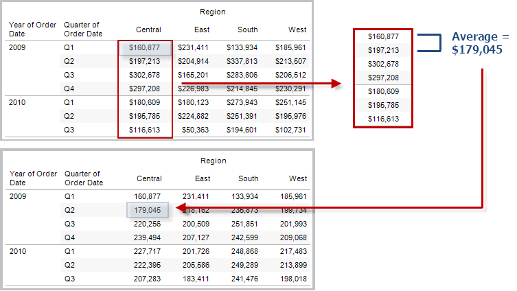
Example
RUNNING_AVG(SUM([Profit])) computes the running average of SUM(Profit).
RUNNING_COUNT(expression)
Returns the running count of the given expression, from the first row in the partition to the current row.
Example
RUNNING_COUNT(SUM([Profit])) computes the running count of SUM(Profit).
RUNNING_MAX(expression)
Returns the running maximum of the given expression, from the first row in the partition to the current row.
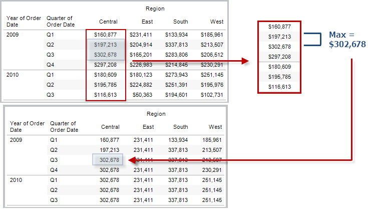
Example
RUNNING_MAX(SUM([Profit])) computes the running maximum of SUM(Profit).
RUNNING_MIN(expression)
Returns the running minimum of the given expression, from the first row in the partition to the current row.
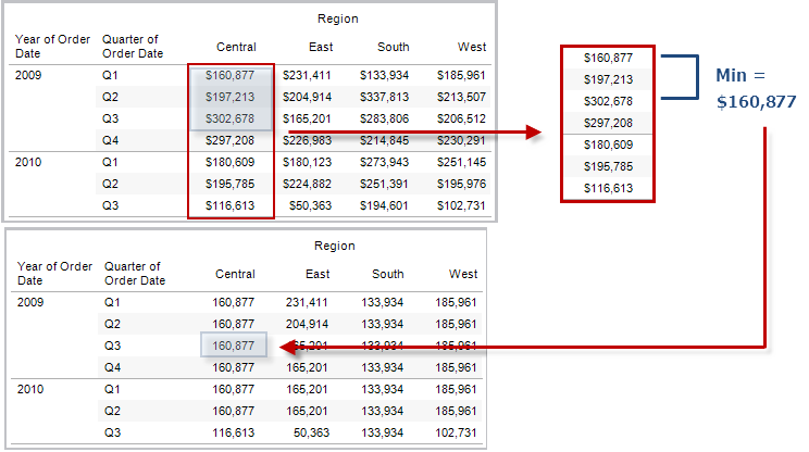
Example
RUNNING_MIN(SUM([Profit])) computes the running minimum of SUM(Profit).
RUNNING_SUM(expression)
Returns the running sum of the given expression, from the first row in the partition to the current row.
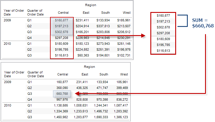
Example
RUNNING_SUM(SUM([Profit])) computes the running sum of SUM(Profit)
SIZE()
Returns the number of rows in the partition. For example, the view below shows quarterly sales. Within the Date partition, there are seven rows, so the Size() of the Date partition is 7.
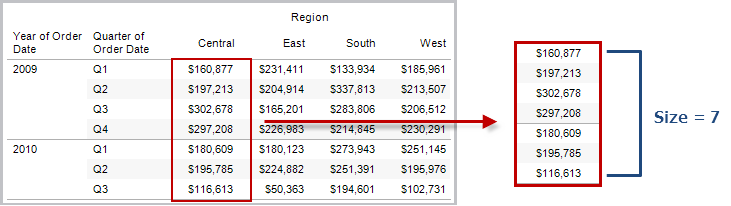
Example
SIZE() = 5 when the current partition contains five rows.
The script functions:
SCRIPT_BOOL
SCRIPT_INT
SCRIPT_REAL
SCRIPT_STRING
are used to pass data to an external service such as R, TabPy or Matlab. See Analytics Extensions(Link opens in a new window).
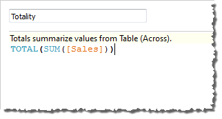
TOTAL(expression)
Returns the total for the given expression in a table calculation partition.
Example
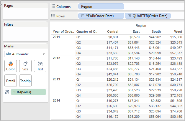
Assume you are starting with this view:
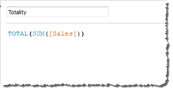
You open the calculation editor and create a new field which you name Totality:
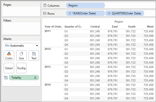
You then drop Totality on Text, to replace SUM(Sales). Your view changes such that it sums values based on the default Compute Using value:
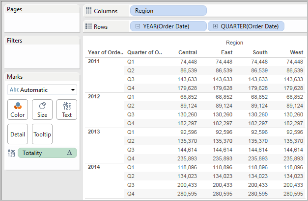
This raises the question, What is the default Compute Using value? If you right-click (Control-click on a Mac) Totality in the Data pane and choose Edit, there is now an additional bit of information available:
The default Compute Using value is Table (Across). The result is that Totality is summing the values across each row of your table. Thus, the value that you see across each row is the sum of the values from the original version of the table.
The values in the 2011/Q1 row in the original table were $8601, $6579, $44262 and $15006. The values in the table after Totality replaces SUM(Sales) are all $74,448, which is the sum of the four original values.
Notice the triangle next to Totality after you drop it on Text:
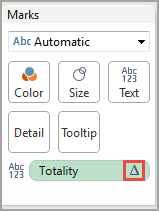
This indicates that this field is using a table calculation. You can right-click the field and choose Edit Table Calculation to redirect your function to a different Compute Using value. For example, you could set it to Table (Down). In that case, your table would look like this:
TOTAL(expression)
Returns the total for the given expression in a table calculation partition.
Example
Assume you are starting with this view:
You open the calculation editor and create a new field which you name Totality:
You then drop Totality on Text, to replace SUM(Sales). Your view changes such that it sums values based on the default Compute Using value:
This raises the question, What is the default Compute Using value? If you right-click (Control-click on a Mac) Totality in the Data pane and choose Edit, there is now an additional bit of information available:
The default Compute Using value is Table (Across). The result is that Totality is summing the values across each row of your table. Thus, the value that you see across each row is the sum of the values from the original version of the table.
The values in the 2011/Q1 row in the original table were $8601, $6579, $44262 and $15006. The values in the table after Totality replaces SUM(Sales) are all $74,448, which is the sum of the four original values.
Notice the triangle next to Totality after you drop it on Text:
This indicates that this field is using a table calculation. You can right-click the field and choose Edit Table Calculation to redirect your function to a different Compute Using value. For example, you could set it to Table (Down). In that case, your table would look like this:
WINDOW_CORR(expression1, expression2, [start, end])
Returns the Pearson correlation coefficient of two expressions within the window. The window is defined as offsets from the current row. Use FIRST()+n and LAST()-n for offsets from the first or last row in the partition. If start and end are omitted, the entire partition is used.
The Pearson correlation measures the linear relationship between two variables. Results range from -1 to +1 inclusive, where 1 denotes an exact positive linear relationship, as when a positive change in one variable implies a positive change of corresponding magnitude in the other, 0 denotes no linear relationship between the variance and - is an exact negative relationship.
There is an equivalent aggregation fuction: CORR. See Tableau Functions (Alphabetical)(Link opens in a new window).
Example
The following formula returns the Pearson correlation of SUM(Profit) and SUM(Sales) from the five previous rows to the current row.
WINDOW_CORR(SUM[Profit]), SUM([Sales]), -5, 0)
WINDOW_COUNT(expression, [start, end])
Returns the count of the expression within the window. The window is defined by means of offsets from the current row. Use FIRST()+n and LAST()-n for offsets from the first or last row in the partition. If the start and end are omitted, the entire partition is used.
Example
WINDOW_COUNT(SUM([Profit]), FIRST()+1, 0) computes the count of SUM(Profit) from the second row to the current row
WINDOW_COVAR(expression1, expression2, [start, end])
Returns the sample covariance of two expressions within the window. The window is defined as offsets from the current row. Use FIRST()+n and LAST()-n for offsets from the first or last row in the partition. If the start and end arguments are omitted, the window is the entire partition.
Sample covariance uses the number of non-null data points n - 1 to normalise the covariance calculation, rather than n, which is used by the population covariance (with the WINDOW_COVARP function). Sample covariance is the appropriate choice when the data is a random sample that is being used to estimate the covariance for a larger population.
There is an equivalent aggregation fuction: COVAR. See Tableau Functions (Alphabetical)(Link opens in a new window).
Example
The following formula returns the sample covariance of SUM(Profit) and SUM(Sales) from the two previous rows to the current row.
WINDOW_COVAR(SUM([Profit]), SUM([Sales]), -2, 0)
WINDOW_COVARP(expression1, expression2, [start, end])
Returns the population covariance of two expressions within the window. The window is defined as offsets from the current row. Use FIRST()+n and LAST()-n for offsets from the first or last row in the partition. If start and end are omitted, the entire partition is used.
Population covariance is sample covariance multiplied by (n-1)/n, where n is the total number of non-null data points. Population covariance is the appropriate choice when there is data available for all items of interest as opposed to when there is only a random subset of items, in which case sample covariance (with the WINDOW_COVAR function) is appropriate.
There is an equivalent aggregation fuction: COVARP. Tableau Functions (Alphabetical)(Link opens in a new window).
Example
The following formula returns the population covariance of SUM(Profit) and SUM(Sales) from the two previous rows to the current row.
WINDOW_COVARP(SUM([Profit]), SUM([Sales]), -2, 0)
WINDOW_MEDIAN(expression, [start, end])
Returns the median of the expression within the window. The window is defined by means of offsets from the current row. Use FIRST()+n and LAST()-n for offsets from the first or last row in the partition. If the start and end are omitted, the entire partition is used.
For example, the view below shows quarterly profit. A window median within the Date partition returns the median profit across all dates.
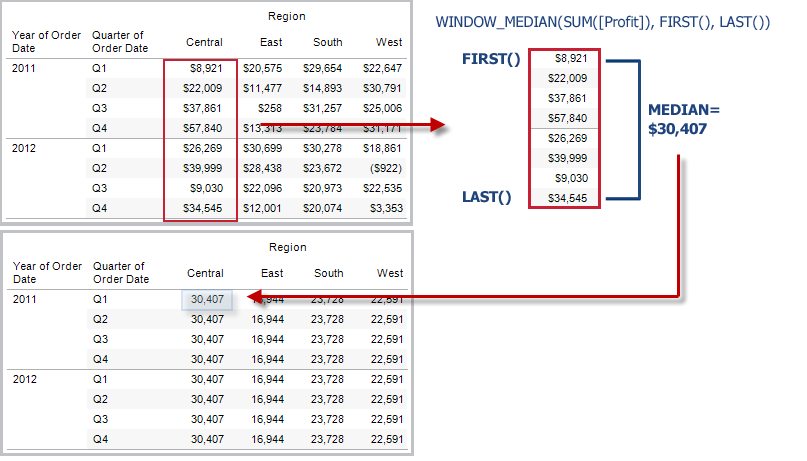
Example
WINDOW_MEDIAN(SUM([Profit]), FIRST()+1, 0) computes the median of SUM(Profit) from the second row to the current row.
WINDOW_MAX(expression, [start, end])
Returns the maximum of the expression within the window. The window is defined by means of offsets from the current row. Use FIRST()+n and LAST()-n for offsets from the first or last row in the partition. If the start and end are omitted, the entire partition is used.
For example, the view below shows quarterly sales. A window maximum within the Date partition returns the maximum sales across all dates.
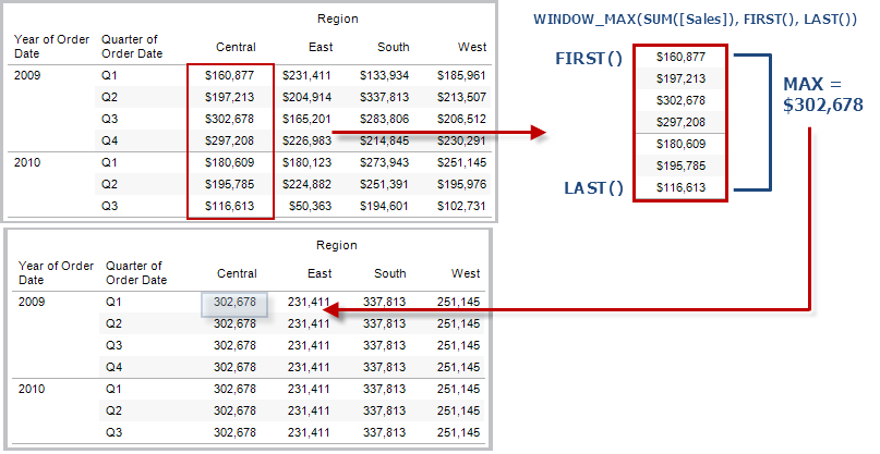
Example
WINDOW_MAX(SUM([Profit]), FIRST()+1, 0) computes the maximum of SUM(Profit) from the second row to the current row.
WINDOW_MIN(expression, [start, end])
Returns the minimum of the expression within the window. The window is defined by means of offsets from the current row. Use FIRST()+n and LAST()-n for offsets from the first or last row in the partition. If the start and end are omitted, the entire partition is used.
For example, the view below shows quarterly sales. A window minimum within the Date partition returns the minimum sales across all dates.
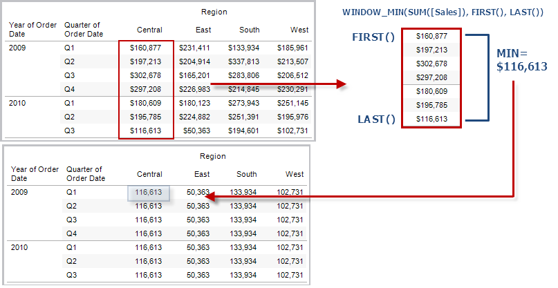
Example
WINDOW_MIN(SUM([Profit]), FIRST()+1, 0) computes the minimum of SUM(Profit) from the second row to the current row.
WINDOW_PERCENTILE(expression, number, [start, end])
Returns the value corresponding to the specified percentile within the window. The window is defined by means of offsets from the current row. Use FIRST()+n and LAST()-n for offsets from the first or last row in the partition. If the start and end are omitted, the entire partition is used.
Example
WINDOW_PERCENTILE(SUM([Profit]), 0.75, -2, 0) returns the 75th percentile for SUM(Profit) from the two previous rows to the current row.
WINDOW_STDEV(expression, [start, end])
Returns the sample standard deviation of the expression within the window. The window is defined by means of offsets from the current row. Use FIRST()+n and LAST()-n for offsets from the first or last row in the partition. If the start and end are omitted, the entire partition is used.
Example
WINDOW_STDEV(SUM([Profit]), FIRST()+1, 0) computes the standard deviation of SUM(Profit) from the second row to the current row.
WINDOW_STDEVP(expression, [start, end])
Returns the biased standard deviation of the expression within the window. The window is defined by means of offsets from the current row. Use FIRST()+n and LAST()-n for offsets from the first or last row in the partition. If the start and end are omitted, the entire partition is used.
Example
WINDOW_STDEVP(SUM([Profit]), FIRST()+1, 0) computes the standard deviation of SUM(Profit) from the second row to the current row.
WINDOW_SUM(expression, [start, end])
Returns the sum of the expression within the window. The window is defined by means of offsets from the current row. Use FIRST()+n and LAST()-n for offsets from the first or last row in the partition. If the start and end are omitted, the entire partition is used.
For example, the view below shows quarterly sales. A window sum computed within the Date partition returns the summation of sales across all quarters.
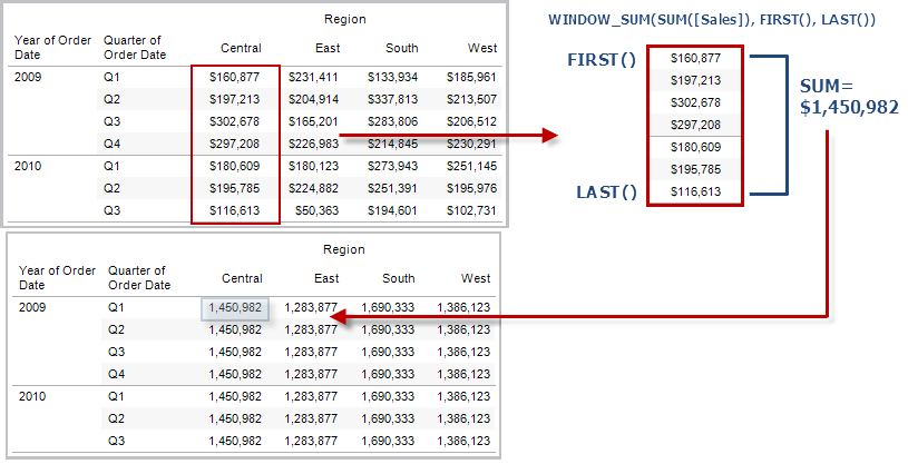
Example
WINDOW_SUM(SUM([Profit]), FIRST()+1, 0) computes the sum of SUM(Profit) from the second row to the current row.
WINDOW_VAR(expression, [start, end])
Returns the sample variance of the expression within the window. The window is defined by means of offsets from the current row. Use FIRST()+n and LAST()-n for offsets from the first or last row in the partition. If the start and end are omitted, the entire partition is used.
Example
WINDOW_VAR((SUM([Profit])), FIRST()+1, 0) computes the variance of SUM(Profit) from the second row to the current row.
WINDOW_VARP(expression, [start, end])
Returns the biased variance of the expression within the window. The window is defined by means of offsets from the current row. Use FIRST()+n and LAST()-n for offsets from the first or last row in the partition. If the start and end are omitted, the entire partition is used.
Example
WINDOW_VARP(SUM([Profit]), FIRST()+1, 0) computes the variance of SUM(Profit) from the second row to the current row.
Analytic Extensions are connections between Tableau and an external service such as TabPy for Python, Matlab and R. To use Analytics Extensions in your analysis, you must first configure a connection(Link opens in a new window) between Tableau and an external service such as a TabPy server. Then you can use scripts inside specific table calculations (MODEL_EXTENSION_ for using published named models, or SCRIPT_ for passing an expression to the external service). The data in the viz (the "table" of the table calc) is passed securely to the external server, the script is run and the results are passed back as the output of the calculation.
Model extension functions
For use with named models deployed on a TabPy external service.
MODEL_EXTENSION_BOOL (model_name, arguments, expression)
Returns the boolean result of an expression as calculated by a named model deployed on a TabPy external service.
Model_name is the name of the deployed analytics model you want to use.
Each argument is a single string that sets the input values that the deployed model accepts and is defined by the analytics model.
Use expressions to define the values that are sent from Tableau to the analytics model. Be sure to use aggregation functions (SUM, AVG, etc.) to aggregate the results.
When using the function, the data types and order of the expressions must match those of the input arguments.
Example
MODEL_EXTENSION_BOOL ("isProfitable","inputSales", "inputCosts", SUM([Sales]), SUM([Costs]))
MODEL_EXTENSION_INT (model_name, arguments, expression)
Returns an integer result of an expression as calculated by a named model deployed on a TabPy external service.
Model_name is the name of the deployed analytics model you want to use.
Each argument is a single string that sets the input values that the deployed model accepts and is defined by the analytics model.
Use expressions to define the values that are sent from Tableau to the analytics model. Be sure to use aggregation functions (SUM, AVG, etc.) to aggregate the results.
When using the function, the data types and order of the expressions must match those of the input arguments.
Example
MODEL_EXTENSION_INT ("getPopulation", "inputCity", "inputState", MAX([City]), MAX ([State]))
MODEL_EXTENSION_REAL (model_name, arguments, expression)
Returns a real result of an expression as calculated by a named model deployed on a TabPy external service.
Model_name is the name of the deployed analytics model you want to use.
Each argument is a single string that sets the input values that the deployed model accepts and is defined by the analytics model.
Use expressions to define the values that are sent from Tableau to the analytics model. Be sure to use aggregation functions (SUM, AVG, etc.) to aggregate the results.
When using the function, the data types and order of the expressions must match those of the input arguments.
Example
MODEL_EXTENSION_REAL ("profitRatio", "inputSales", "inputCosts", SUM([Sales]), SUM([Costs]))
MODEL_EXTENSION_STRING (model_name, arguments, expression)
Returns the string result of an expression as calculated by a named model deployed on a TabPy external service.
Model_name is the name of the deployed analytics model you want to use.
Each argument is a single string that sets the input values that the deployed model accepts and is defined by the analytics model.
Use expressions to define the values that are sent from Tableau to the analytics model. Be sure to use aggregation functions (SUM, AVG, etc.) to aggregate the results.
When using the function, the data types and order of the expressions must match those of the input arguments.
Example
MODEL_EXTENSION_STR ("mostPopulatedCity", "inputCountry", "inputYear", MAX ([Country]), MAX([Year]))
Script functions
Instead of using a defined external model like MODEL_EXPRESSION functions, SCRIPT functions are used to specify the expression directly in the table calculation.
Returns a Boolean result from the specified expression. The expression is passed directly to a running analytics extension service instance.
In R expressions, use .argn (with a leading dot) to reference parameters (.arg1, .arg2, etc.).
In Python expressions, use _argn (with a leading underscore).
Examples
In this R example, .arg1 is equal to SUM([Profit]):
SCRIPT_BOOL("is.finite(.arg1)", SUM([Profit]))
The next example returns True for store IDs in Washington state, and False otherwise. This example could be the definition for a calculated field titled IsStoreInWA.
SCRIPT_BOOL('grepl(".*_WA", .arg1, perl=TRUE)',ATTR([Store ID]))
A command for Python would take this form:
SCRIPT_BOOL("return map(lambda x : x > 0, _arg1)", SUM([Profit]))
SCRIPT_INT
Returns an integer result from the specified expression. The expression is passed directly to a running analytics extension service instance.
In R expressions, use .argn (with a leading dot) to reference parameters (.arg1, .arg2, etc.)
In Python expressions, use _argn (with a leading underscore).
Examples
In this R example, .arg1 is equal to SUM([Profit]):
SCRIPT_INT("is.finite(.arg1)", SUM([Profit]))
In the next example, k-means clustering is used to create three clusters:
SCRIPT_INT('result <- kmeans(data.frame(.arg1,.arg2,.arg3,.arg4), 3);result$cluster;', SUM([Petal length]), SUM([Petal width]),SUM([Sepal length]),SUM([Sepal width]))
A command for Python would take this form:
SCRIPT_INT("return map(lambda x : int(x * 5), _arg1)", SUM([Profit]))
SCRIPT_REAL
Returns a real result from the specified expression. The expression is passed directly to a running analytics extension service instance. In
R expressions, use .argn (with a leading dot) to reference parameters (.arg1, .arg2, etc.)
In Python expressions, use _argn (with a leading underscore).
Examples
In this R example, .arg1 is equal to SUM([Profit]):
SCRIPT_REAL("is.finite(.arg1)", SUM([Profit]))
The next example converts temperature values from Celsius to Fahrenheit.
SCRIPT_REAL('library(udunits2);ud.convert(.arg1, "celsius", "degree_fahrenheit")',AVG([Temperature]))
A command for Python would take this form:
SCRIPT_REAL("return map(lambda x : x * 0.5, _arg1)", SUM([Profit]))
SCRIPT_STR
Returns a string result from the specified expression. The expression is passed directly to a running analytics extension service instance.
In R expressions, use .argn (with a leading dot) to reference parameters (.arg1, .arg2, etc.)
In Python expressions, use _argn (with a leading underscore).
Examples
In this R example, .arg1 is equal to SUM([Profit]):
SCRIPT_STR("is.finite(.arg1)", SUM([Profit]))
The next example extracts a state abbreviation from a more complicated string (in the original form 13XSL_CA, A13_WA):
SCRIPT_STR('gsub(".*_", "", .arg1)',ATTR([Store ID]))
A command for Python would take this form:
SCRIPT_STR("return map(lambda x : x[:2], _arg1)", ATTR([Region]))
Follow along with the steps below to learn how to create a table calculation using the calculation editor.
Note: There are several ways to create table calculations in Tableau. This example demonstrates only one of those ways. For more information, see Transform Values with Table Calculations(Link opens in a new window).
Step 1: Create the visualisation
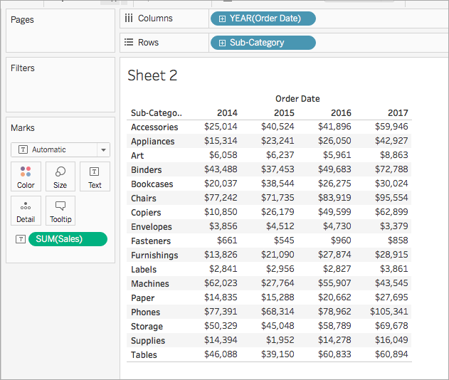
In Tableau Desktop, connect to the Sample-Superstore saved data source, which comes with Tableau.
Navigate to a worksheet.
From the Data pane, under Dimensions, drag Order Date to the Columns shelf.
From the Data pane, under Dimensions, drag Sub-Category to the Rows shelf.
From the Data pane, under Measures, drag Sales to Text on the Marks card.
Your visualisation updates to a text table.
Step 2: Create the table calculation
Select Analysis > Create Calculated Field.
In the calculation editor that opens, do the following:
- Name the calculated field, Running Sum of Profit.
Enter the following formula:
RUNNING_SUM(SUM([Profit]))This formula calculates the running sum of profit sales. It is computed across the entire table.
When finished, click OK.
The new table calculation field appears under Measures in the Data pane. Just like your other fields, you can use it in one or more visualisations.
Step 3: Use the table calculation in the visualisation
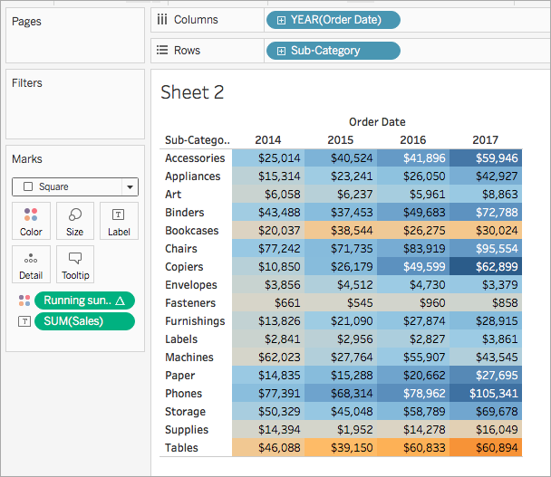
From the Data pane, under Measures, drag Running Sum of Profit to Colour on the Marks card.
On the Marks card, click the Mark Type drop-down and select Square.
The visualisation updates to a highlight table:
Step 4: Edit the table calculation
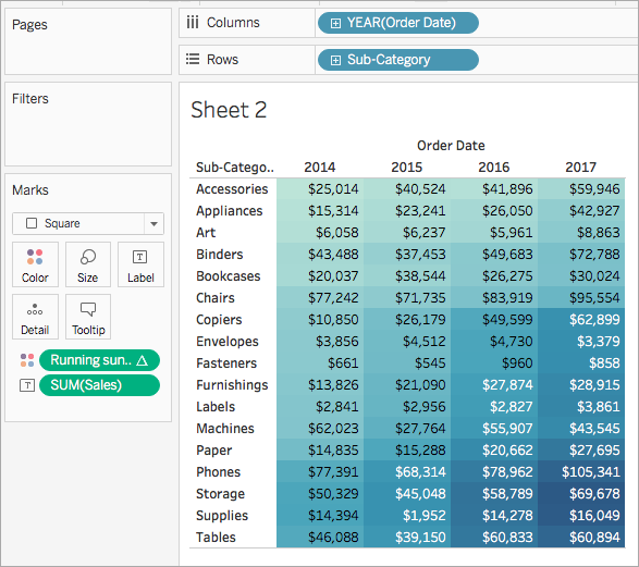
- On the Marks card, right-click Running Sum of Profit and select Edit Table Calculation.
In the Table Calculation dialog box that opens, under Compute Using, select Table (down).
The visualisation updates to the following:
See Also
Create a table calculation(Link opens in a new window)
Customise Table Calculations(Link opens in a new window)